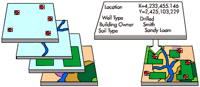
GIS with  and
and  
Getting some data
There are many sources of GIS data. Here are some useful links:
- WorldMap
- FAO's GeoNetwork
- IPUMS USA Boundary files for Censuses
- IPUMS International Boundary files for Censuses
- GADM database of Global Administrative Areas
- Global Administrative Unit Layers
- Natural Earth: All kinds of geographical, cultural and socioeconomic variables
- Global Map
- Digital Chart of the World
- Sage and Sage Atlas
- Caloric Suitability Index CSI: Agricultural suitability data
- Ramankutti's Datasets on land use, crops, etc.
- SEDAC at Columbia Univesrity: Gridded Population, Hazzards, etc.
- World Port Index
- USGS elevation maps
- NOOA's Global Land One-km Base Elevation Project (GLOBE)
- NOOA Nightlight data: This is the data used by Henderson, Storeygard, and Weil AER 2012 paper.
- Other NOOA Data
- GEcon
- OpenStreetMap
- U.S. Census TIGER
- Geo-referencing of Ethnic Groups
See also Wikipedia links
Set-up
Let's import the packages we will use and set the paths for outputs.
# Let's import pandas and some other basic packages we will use
from __future__ import division
%pylab --no-import-all
%matplotlib inline
import pandas as pd
import numpy as np
import os, sys
Using matplotlib backend: <object object at 0x1164f0770>
%pylab is deprecated, use %matplotlib inline and import the required libraries.
Populating the interactive namespace from numpy and matplotlib
# GIS packages
import geopandas as gpd
from geopandas.tools import overlay
from shapely.geometry import Polygon, Point
import georasters as gr
# Alias for Geopandas
gp = gpd
# Plotting
import matplotlib as mpl
import seaborn as sns
# Setup seaborn
sns.set()
# Paths
pathout = './data/'

if not os.path.exists(pathout):
    os.mkdir(pathout)

pathgraphs = './graphs/'
if not os.path.exists(pathgraphs):
    os.mkdir(pathgraphs)
Initial Example -- Natural Earth Country Shapefile
Let's download a shapefile with all the polygons for countries so we can visualize and analyze some of the data we have downloaded in other notebooks. Natural Earth provides lots of free data so let's use that one.
For shapefiles and other polygon type data geopandas is the most useful package. geopandas is to GIS what pandas is to other data. Since gepandas extends the functionality of pandas to a GIS dataset, all the nice functions and properties of pandas are also available in geopandas. Of course, geopandas includes functions and properties unique to GIS data.
Next we will use it to download the shapefile (which is contained in a zip archive). geopandas extends pandas for use with GIS data. We can use many functions and properties of the GeoDataFrame to analyze our data.
import requests
import io

#headers = {'User-Agent': 'Mozilla/5.0 (Macintosh; Intel Mac OS X 10_10_1) AppleWebKit/537.36 (KHTML, like Gecko) Chrome/39.0.2171.95 Safari/537.36'}
headers = {'User-Agent': 'Mozilla/5.0 (X11; Linux x86_64) AppleWebKit/537.36 (KHTML, like Gecko) Chrome/51.0.2704.103 Safari/537.36', 'Accept': 'text/html,application/xhtml+xml,application/xml;q=0.9,*/*;q=0.8'}

url = 'https://naturalearth.s3.amazonaws.com/10m_cultural/ne_10m_admin_0_countries.zip'
r = requests.get(url, headers=headers)
countries = gp.read_file(io.BytesIO(r.content))
#countries = gpd.read_file('https://www.naturalearthdata.com/http//www.naturalearthdata.com/download/10m/cultural/ne_10m_admin_0_countries.zip')
Let's look inside this GeoDataFrame
countries.head(10)
| featurecla | scalerank | LABELRANK | SOVEREIGNT | SOV_A3 | ADM0_DIF | LEVEL | TYPE | TLC | ADMIN | ... | FCLASS_TR | FCLASS_ID | FCLASS_PL | FCLASS_GR | FCLASS_IT | FCLASS_NL | FCLASS_SE | FCLASS_BD | FCLASS_UA | geometry | |
|---|---|---|---|---|---|---|---|---|---|---|---|---|---|---|---|---|---|---|---|---|---|
| 0 | Admin-0 country | 0 | 2 | Indonesia | IDN | 0 | 2 | Sovereign country | 1 | Indonesia | ... | None | None | None | None | None | None | None | None | None | MULTIPOLYGON (((117.70361 4.16341, 117.70361 4... |
| 1 | Admin-0 country | 0 | 3 | Malaysia | MYS | 0 | 2 | Sovereign country | 1 | Malaysia | ... | None | None | None | None | None | None | None | None | None | MULTIPOLYGON (((117.70361 4.16341, 117.69711 4... |
| 2 | Admin-0 country | 0 | 2 | Chile | CHL | 0 | 2 | Sovereign country | 1 | Chile | ... | None | None | None | None | None | None | None | None | None | MULTIPOLYGON (((-69.51009 -17.50659, -69.50611... |
| 3 | Admin-0 country | 0 | 3 | Bolivia | BOL | 0 | 2 | Sovereign country | 1 | Bolivia | ... | None | None | None | None | None | None | None | None | None | POLYGON ((-69.51009 -17.50659, -69.51009 -17.5... |
| 4 | Admin-0 country | 0 | 2 | Peru | PER | 0 | 2 | Sovereign country | 1 | Peru | ... | None | None | None | None | None | None | None | None | None | MULTIPOLYGON (((-69.51009 -17.50659, -69.63832... |
| 5 | Admin-0 country | 0 | 2 | Argentina | ARG | 0 | 2 | Sovereign country | 1 | Argentina | ... | None | None | None | None | None | None | None | None | None | MULTIPOLYGON (((-67.19390 -22.82222, -67.14269... |
| 6 | Admin-0 country | 3 | 3 | United Kingdom | GB1 | 1 | 2 | Dependency | 1 | Dhekelia Sovereign Base Area | ... | Admin-0 dependency | None | Admin-0 dependency | Admin-0 dependency | Admin-0 dependency | Admin-0 dependency | Admin-0 dependency | None | Admin-0 dependency | POLYGON ((33.78094 34.97635, 33.76043 34.97968... |
| 7 | Admin-0 country | 1 | 5 | Cyprus | CYP | 0 | 2 | Sovereign country | 1 | Cyprus | ... | None | None | None | None | None | None | None | None | None | MULTIPOLYGON (((33.78183 34.97622, 33.78094 34... |
| 8 | Admin-0 country | 0 | 2 | India | IND | 0 | 2 | Sovereign country | 1 | India | ... | None | None | None | None | None | None | None | None | None | MULTIPOLYGON (((77.80035 35.49541, 77.81533 35... |
| 9 | Admin-0 country | 0 | 2 | China | CH1 | 1 | 2 | Country | 1 | China | ... | None | None | None | None | None | None | None | None | None | MULTIPOLYGON (((78.91769 33.38626, 78.91595 33... |
10 rows × 169 columns
Each row contains the information for one country.
Each column is one property or variable.
Unlike pandas DataFrames, geopandas always must have a geometry column.
Let's plot this data
%matplotlib inline
fig, ax = plt.subplots(figsize=(15,10))
countries.plot(ax=ax)
ax.set_title("WGS84 (lat/lon)", fontdict={'fontsize':34})
Text(0.5, 1.0, 'WGS84 (lat/lon)')

We can also get some additional information on this data. For example its projection
countries.crs
<Geographic 2D CRS: EPSG:4326>
Name: WGS 84
Axis Info [ellipsoidal]:
- Lat[north]: Geodetic latitude (degree)
- Lon[east]: Geodetic longitude (degree)
Area of Use:
- name: World.
- bounds: (-180.0, -90.0, 180.0, 90.0)
Datum: World Geodetic System 1984 ensemble
- Ellipsoid: WGS 84
- Prime Meridian: Greenwich
We can reproject the data from its current WGS84 projection to other ones. Let's do this and plot the results so we can see how different projections distort results.
fig, ax = plt.subplots(figsize=(15,10))
countries_merc = countries.to_crs(epsg=3857)
countries_merc.loc[countries_merc.NAME!='Antarctica'].reset_index().plot(ax=ax)
ax.set_title("Mercator", fontdict={'fontsize':34})
Text(0.5, 1.0, 'Mercator')

countries_merc.crs
<Projected CRS: EPSG:3857>
Name: WGS 84 / Pseudo-Mercator
Axis Info [cartesian]:
- X[east]: Easting (metre)
- Y[north]: Northing (metre)
Area of Use:
- name: World between 85.06°S and 85.06°N.
- bounds: (-180.0, -85.06, 180.0, 85.06)
Coordinate Operation:
- name: Popular Visualisation Pseudo-Mercator
- method: Popular Visualisation Pseudo Mercator
Datum: World Geodetic System 1984 ensemble
- Ellipsoid: WGS 84
- Prime Meridian: Greenwich
cea = {'datum': 'WGS84',
 'lat_ts': 0,
 'lon_0': 0,
 'no_defs': True,
 'over': True,
 'proj': 'cea',
 'units': 'm',
 'x_0': 0,
 'y_0': 0}

cea = 'ESRI:54034'
fig, ax = plt.subplots(figsize=(15,10))
countries_cea = countries.to_crs(crs=cea)
countries_cea.plot(ax=ax)
ax.set_title("Cylindrical Equal Area", fontdict={'fontsize':34})
Text(0.5, 1.0, 'Cylindrical Equal Area')

countries_cea.crs
<Projected CRS: ESRI:54034>
Name: World_Cylindrical_Equal_Area
Axis Info [cartesian]:
- E[east]: Easting (metre)
- N[north]: Northing (metre)
Area of Use:
- name: World.
- bounds: (-180.0, -90.0, 180.0, 90.0)
Coordinate Operation:
- name: World_Cylindrical_Equal_Area
- method: Lambert Cylindrical Equal Area
Datum: World Geodetic System 1984
- Ellipsoid: WGS 84
- Prime Meridian: Greenwich
Notice that each projection shows the world in a very different manner, distoring areas, distances etc. So you need to take care when doing computations to use the correct projection. An important issue to remember is that you need a projected (not geographical) projection to compute areas and distances. Let's compare these three a bit. Start with the boundaries of each.
print('[xmin, ymin, xmax, ymax] in three projections')
print(countries.total_bounds)
print(countries_merc.total_bounds)
print(countries_cea.total_bounds)
[xmin, ymin, xmax, ymax] in three projections
[-180.          -90.          180.           83.63410065]
[-2.00375083e+07 -2.25045148e+08  2.00375083e+07  1.84289200e+07]
[-20037508.34278923  -6363885.33192604  20037508.34278924
   6324296.52646162]
Let's describe the areas of these countries in the three projections
print('Area distribution in WGS84')
print(countries.area.describe(), '\n')
Area distribution in WGS84
count     258.000000
mean       83.053683
std       443.786684
min         0.000001
25%         0.065859
50%         5.857276
75%        37.279026
max      6049.574693
dtype: float64
/var/folders/2r/7vb_23y1427bffj2wbz7mxfc0000gq/T/ipykernel_69226/1371744286.py:2: UserWarning: Geometry is in a geographic CRS. Results from 'area' are likely incorrect. Use 'GeoSeries.to_crs()' to re-project geometries to a projected CRS before this operation.

  print(countries.area.describe(), '\n')
print('Area distribution in Mercator')
print(countries_merc.area.describe(), '\n')
Area distribution in Mercator
count    2.580000e+02
mean     3.423154e+13
std      5.295922e+14
min      2.204709e+04
25%      9.801617e+08
50%      8.692411e+10
75%      5.411109e+11
max      8.507102e+15
dtype: float64
print('Area distribution in CEA')
print(countries_cea.area.describe(), '\n')
Area distribution in CEA
count    2.580000e+02
mean     5.690945e+11
std      1.826917e+12
min      1.220383e+04
25%      6.986665e+08
50%      5.148888e+10
75%      3.544773e+11
max      1.698019e+13
dtype: float64
countries['geometry']
0      MULTIPOLYGON (((117.70361 4.16341, 117.70361 4...
1      MULTIPOLYGON (((117.70361 4.16341, 117.69711 4...
2      MULTIPOLYGON (((-69.51009 -17.50659, -69.50611...
3      POLYGON ((-69.51009 -17.50659, -69.51009 -17.5...
4      MULTIPOLYGON (((-69.51009 -17.50659, -69.63832...
                             ...
253    MULTIPOLYGON (((113.55860 22.16303, 113.56943 ...
254    POLYGON ((123.59702 -12.42832, 123.59775 -12.4...
255    POLYGON ((-79.98929 15.79495, -79.98782 15.796...
256    POLYGON ((-78.63707 15.86209, -78.64041 15.864...
257    POLYGON ((117.75389 15.15437, 117.75569 15.151...
Name: geometry, Length: 258, dtype: geometry
Point((0,0))

Polygon(((0,0), (1,2), (3,0)))

Let's compare the area of each country in the two projected projections
countries_merc = countries_merc.set_index('ADM0_A3')
countries_cea = countries_cea.set_index('ADM0_A3')
countries_merc['ratio_area'] = countries_merc.area / countries_cea.area
countries_cea['ratio_area'] = countries_merc.area / countries_cea.area
sns.set(rc={'figure.figsize':(11.7,8.27)})
sns.set_context("talk")
fig, ax = plt.subplots()
sns.scatterplot(x=countries_cea.area/1e6, y=countries_merc.area/1e6, ax=ax)
sns.lineplot(x=countries_cea.area/1e6, y=countries_cea.area/1e6, color='r', ax=ax)
ax.set_ylabel('Mercator')
ax.set_xlabel('CEA')
ax.set_title("Areas")
Text(0.5, 1.0, 'Areas')

Now, how do we know what is correct? Let's get some data from WDI to compare the areas of countries in these projections to what the correct area should be (notice that each country usually will use a local projection that ensures areas are correctly computed, so their data should be closer to the truth than any of our global ones).
Here we use some of what we learned before in this notebook.
from pandas_datareader import data, wb
wbcountries = wb.get_countries()
wbcountries['name'] = wbcountries.name.str.strip()
wdi = wb.download(indicator=['AG.LND.TOTL.K2'], country=wbcountries.iso2c.values, start=2017, end=2017)
wdi.columns = ['WDI_area']
wdi = wdi.reset_index()
wdi = wdi.merge(wbcountries[['iso3c', 'iso2c', 'name']], left_on='country', right_on='name')

countries_cea['CEA_area'] = countries_cea.area / 1e6
countries_merc['MERC_area'] = countries_merc.area / 1e6
areas = pd.merge(countries_cea['CEA_area'], countries_merc['MERC_area'], left_index=True, right_index=True)
/Users/ozak/miniforge3/envs/GeoPython311env/lib/python3.11/site-packages/pandas_datareader/wb.py:592: UserWarning: Non-standard ISO country codes: 1A, 1W, 4E, 6F, 6N, 6X, 7E, 8S, A4, A5, A9, B1, B2, B3, B4, B6, B7, B8, C4, C5, C6, C7, C8, C9, D2, D3, D4, D5, D6, D7, EU, F1, F6, JG, M1, M2, N6, OE, R6, S1, S2, S3, S4, T2, T3, T4, T5, T6, T7, V1, V2, V3, V4, XC, XD, XE, XF, XG, XH, XI, XJ, XK, XL, XM, XN, XO, XP, XQ, XT, XU, XY, Z4, Z7, ZB, ZF, ZG, ZH, ZI, ZJ, ZQ, ZT
  warnings.warn(
/var/folders/2r/7vb_23y1427bffj2wbz7mxfc0000gq/T/ipykernel_69226/2997326858.py:4: FutureWarning: errors='ignore' is deprecated and will raise in a future version. Use to_numeric without passing `errors` and catch exceptions explicitly instead
  wdi = wb.download(indicator=['AG.LND.TOTL.K2'], country=wbcountries.iso2c.values, start=2017, end=2017)
Let's merge the WDI data with what we have computed before.
wdi = wdi.merge(areas, left_on='iso3c', right_index=True)
wdi
| country | year | WDI_area | iso3c | iso2c | name | CEA_area | MERC_area | |
|---|---|---|---|---|---|---|---|---|
| 0 | Aruba | 2017 | 180.0 | ABW | AW | Aruba | 1.697662e+02 | 1.792215e+02 |
| 2 | Afghanistan | 2017 | 652230.0 | AFG | AF | Afghanistan | 6.421811e+05 | 9.349973e+05 |
| 4 | Angola | 2017 | 1246700.0 | AGO | AO | Angola | 1.244652e+06 | 1.316011e+06 |
| 5 | Albania | 2017 | 27400.0 | ALB | AL | Albania | 2.833579e+04 | 5.002434e+04 |
| 6 | Andorra | 2017 | 470.0 | AND | AD | Andorra | 4.522394e+02 | 8.335608e+02 |
| ... | ... | ... | ... | ... | ... | ... | ... | ... |
| 260 | Samoa | 2017 | 2780.0 | WSM | WS | Samoa | 2.780425e+03 | 2.964662e+03 |
| 262 | Yemen, Rep. | 2017 | 527970.0 | YEM | YE | Yemen, Rep. | 4.530748e+05 | 4.929999e+05 |
| 263 | South Africa | 2017 | 1213090.0 | ZAF | ZA | South Africa | 1.219825e+06 | 1.605941e+06 |
| 264 | Zambia | 2017 | 743390.0 | ZMB | ZM | Zambia | 7.519143e+05 | 8.011173e+05 |
| 265 | Zimbabwe | 2017 | 386850.0 | ZWE | ZW | Zimbabwe | 3.893382e+05 | 4.382042e+05 |
213 rows × 8 columns
How correlated are these measures?
wdi.corr(numeric_only=True)
| WDI_area | CEA_area | MERC_area | |
|---|---|---|---|
| WDI_area | 1.000000 | 0.997195 | 0.822258 |
| CEA_area | 0.997195 | 1.000000 | 0.852868 |
| MERC_area | 0.822258 | 0.852868 | 1.000000 |
Let's change the shape of the data so we can plot it using seaborn.
wdi2 = wdi.melt(id_vars=['iso3c', 'iso2c', 'name', 'country', 'year', 'WDI_area'], value_vars=['CEA_area', 'MERC_area'])
wdi2
| iso3c | iso2c | name | country | year | WDI_area | variable | value | |
|---|---|---|---|---|---|---|---|---|
| 0 | ABW | AW | Aruba | Aruba | 2017 | 180.0 | CEA_area | 1.697662e+02 |
| 1 | AFG | AF | Afghanistan | Afghanistan | 2017 | 652230.0 | CEA_area | 6.421811e+05 |
| 2 | AGO | AO | Angola | Angola | 2017 | 1246700.0 | CEA_area | 1.244652e+06 |
| 3 | ALB | AL | Albania | Albania | 2017 | 27400.0 | CEA_area | 2.833579e+04 |
| 4 | AND | AD | Andorra | Andorra | 2017 | 470.0 | CEA_area | 4.522394e+02 |
| ... | ... | ... | ... | ... | ... | ... | ... | ... |
| 421 | WSM | WS | Samoa | Samoa | 2017 | 2780.0 | MERC_area | 2.964662e+03 |
| 422 | YEM | YE | Yemen, Rep. | Yemen, Rep. | 2017 | 527970.0 | MERC_area | 4.929999e+05 |
| 423 | ZAF | ZA | South Africa | South Africa | 2017 | 1213090.0 | MERC_area | 1.605941e+06 |
| 424 | ZMB | ZM | Zambia | Zambia | 2017 | 743390.0 | MERC_area | 8.011173e+05 |
| 425 | ZWE | ZW | Zimbabwe | Zimbabwe | 2017 | 386850.0 | MERC_area | 4.382042e+05 |
426 rows × 8 columns
sns.set(rc={'figure.figsize':(11.7,8.27)})
sns.set_context("talk")
fig, ax = plt.subplots()
sns.scatterplot(x='WDI_area', y='value', data=wdi2, hue='variable', ax=ax)
#sns.scatterplot(x='WDI_area', y='MERC_area', data=wdi, ax=ax)
sns.lineplot(x='WDI_area', y='WDI_area', data=wdi, color='r', ax=ax)
ax.set_ylabel('Other')
ax.set_xlabel('WDI')
ax.set_title("Areas")
ax.legend()
<matplotlib.legend.Legend at 0x143adbc90>

We could use other data to compare, e.g. data from the CIA Factbook.
cia_area = pd.read_csv('https://web.archive.org/web/20201116182145if_/https://www.cia.gov/LIBRARY/publications/the-world-factbook/rankorder/rawdata_2147.txt', sep='\t', header=None)
cia_area = pd.DataFrame(cia_area[0].str.strip().str.split('\s\s+').tolist(), columns=['id', 'Name', 'area'])
cia_area.area = cia_area.area.str.replace(',', '').astype(int)
cia_area
| id | Name | area | |
|---|---|---|---|
| 0 | 1 | Russia | 17098242 |
| 1 | 2 | Antarctica | 14000000 |
| 2 | 3 | Canada | 9984670 |
| 3 | 4 | United States | 9833517 |
| 4 | 5 | China | 9596960 |
| ... | ... | ... | ... |
| 249 | 250 | Spratly Islands | 5 |
| 250 | 251 | Ashmore and Cartier Islands | 5 |
| 251 | 252 | Coral Sea Islands | 3 |
| 252 | 253 | Monaco | 2 |
| 253 | 254 | Holy See (Vatican City) | 0 |
254 rows × 3 columns
print('CEA area for Russia', countries_cea.area.loc['RUS'] / 1e6)
print('MERC area for Russia', countries_merc.area.loc['RUS'] / 1e6)
print('WDI area for Russia', wdi.loc[wdi.iso3c=='RUS', 'WDI_area'])
print('CIA area for Russia', cia_area.loc[cia_area.Name=='Russia', 'area'])
CEA area for Russia 16980189.52844945
MERC area for Russia 82997412.6652339
WDI area for Russia 202    16376870.0
Name: WDI_area, dtype: float64
CIA area for Russia 0    17098242
Name: area, dtype: int64
Again very similar result. CEA is closest to both WDI and CIA.
Exercise
- Merge the
CIAdata with the wdi data. You need to get correct codes for the countries to allow for the merge or correct the names to ensure they are compatible. - Change the dataframe as we did with
wdi2and plot the association between these measures
Mapping data
Let's use the geoplot package to plot data in a map. As usual we can do it in many ways, but geoplot makes our life very easy. Let's import the various packages we will use.
import geoplot as gplt
import geoplot.crs as gcrs
import mapclassify as mc
import textwrap
Let's import some of the data we had downloaded before. Specifically, let's import the Penn World Tables data.
pwt = pd.read_stata(pathout + 'pwt.dta')
pwt_xls = pd.read_excel(pathout + 'pwt.xlsx')
pwt
| countrycode | country | currency_unit | year | rgdpe | rgdpo | pop | emp | avh | hc | ... | csh_x | csh_m | csh_r | pl_c | pl_i | pl_g | pl_x | pl_m | pl_n | pl_k | |
|---|---|---|---|---|---|---|---|---|---|---|---|---|---|---|---|---|---|---|---|---|---|
| 0 | ABW | Aruba | Aruban Guilder | 1950 | NaN | NaN | NaN | NaN | NaN | NaN | ... | NaN | NaN | NaN | NaN | NaN | NaN | NaN | NaN | NaN | NaN |
| 1 | ABW | Aruba | Aruban Guilder | 1951 | NaN | NaN | NaN | NaN | NaN | NaN | ... | NaN | NaN | NaN | NaN | NaN | NaN | NaN | NaN | NaN | NaN |
| 2 | ABW | Aruba | Aruban Guilder | 1952 | NaN | NaN | NaN | NaN | NaN | NaN | ... | NaN | NaN | NaN | NaN | NaN | NaN | NaN | NaN | NaN | NaN |
| 3 | ABW | Aruba | Aruban Guilder | 1953 | NaN | NaN | NaN | NaN | NaN | NaN | ... | NaN | NaN | NaN | NaN | NaN | NaN | NaN | NaN | NaN | NaN |
| 4 | ABW | Aruba | Aruban Guilder | 1954 | NaN | NaN | NaN | NaN | NaN | NaN | ... | NaN | NaN | NaN | NaN | NaN | NaN | NaN | NaN | NaN | NaN |
| ... | ... | ... | ... | ... | ... | ... | ... | ... | ... | ... | ... | ... | ... | ... | ... | ... | ... | ... | ... | ... | ... |
| 12805 | ZWE | Zimbabwe | US Dollar | 2015 | 40141.617188 | 39798.644531 | 13.814629 | 6.393752 | NaN | 2.584653 | ... | 0.140172 | -0.287693 | -0.051930 | 0.479228 | 0.651287 | 0.541446 | 0.616689 | 0.533235 | 0.425715 | 1.778124 |
| 12806 | ZWE | Zimbabwe | US Dollar | 2016 | 41875.203125 | 40963.191406 | 14.030331 | 6.504374 | NaN | 2.616257 | ... | 0.131920 | -0.251232 | -0.016258 | 0.470640 | 0.651027 | 0.539631 | 0.619789 | 0.519718 | 0.419446 | 1.728804 |
| 12807 | ZWE | Zimbabwe | US Dollar | 2017 | 44672.175781 | 44316.742188 | 14.236595 | 6.611773 | NaN | 2.648248 | ... | 0.126722 | -0.202827 | -0.039897 | 0.473560 | 0.639560 | 0.519956 | 0.619739 | 0.552042 | 0.418681 | 1.756007 |
| 12808 | ZWE | Zimbabwe | US Dollar | 2018 | 44325.109375 | 43420.898438 | 14.438802 | 6.714952 | NaN | 2.680630 | ... | 0.144485 | -0.263658 | -0.020791 | 0.543757 | 0.655473 | 0.529867 | 0.641361 | 0.561526 | 0.426527 | 1.830088 |
| 12809 | ZWE | Zimbabwe | US Dollar | 2019 | 42296.062500 | 40826.570312 | 14.645468 | 6.831017 | NaN | 2.713408 | ... | 0.213562 | -0.270959 | -0.089798 | 0.494755 | 0.652439 | 0.500927 | 0.487763 | 0.430082 | 0.419883 | 1.580885 |
12810 rows × 52 columns
Let's recreate GDPpc data
# Get columns with GDP measures
gdpcols = pwt_xls.loc[pwt_xls['Variable definition'].apply(lambda x: str(x).upper().find('REAL GDP')!=-1), 'Variable name'].tolist()

# Generate GDPpc for each measure
for gdp in gdpcols:
    pwt[gdp + '_pc'] = pwt[gdp] / pwt['pop']

# GDPpc data
gdppccols = [col+'_pc' for col in gdpcols]
pwt[['countrycode', 'country', 'year'] + gdppccols]
| countrycode | country | year | rgdpe_pc | rgdpo_pc | cgdpe_pc | cgdpo_pc | rgdpna_pc | |
|---|---|---|---|---|---|---|---|---|
| 0 | ABW | Aruba | 1950 | NaN | NaN | NaN | NaN | NaN |
| 1 | ABW | Aruba | 1951 | NaN | NaN | NaN | NaN | NaN |
| 2 | ABW | Aruba | 1952 | NaN | NaN | NaN | NaN | NaN |
| 3 | ABW | Aruba | 1953 | NaN | NaN | NaN | NaN | NaN |
| 4 | ABW | Aruba | 1954 | NaN | NaN | NaN | NaN | NaN |
| ... | ... | ... | ... | ... | ... | ... | ... | ... |
| 12805 | ZWE | Zimbabwe | 2015 | 2905.732553 | 2880.905780 | 2892.674328 | 2856.095690 | 3040.848887 |
| 12806 | ZWE | Zimbabwe | 2016 | 2984.619759 | 2919.616893 | 2970.770578 | 2912.558803 | 3016.730437 |
| 12807 | ZWE | Zimbabwe | 2017 | 3137.841301 | 3112.875107 | 3137.841301 | 3112.875107 | 3112.875107 |
| 12808 | ZWE | Zimbabwe | 2018 | 3069.860600 | 3007.236919 | 3071.061791 | 3017.391036 | 3217.517468 |
| 12809 | ZWE | Zimbabwe | 2019 | 2887.996649 | 2787.658975 | 2889.980517 | 2805.080907 | 2915.172824 |
12810 rows × 8 columns
Let's map GDPpc for the year 2010 using geoplot. For this, let's write two functions that will simplify plotting and saving maps. Also, we can reuse it whenever we need to create a new map for the world.
# Functions for plotting
def center_wrap(text, cwidth=32, **kw):
    '''Center Text (to be used in legend)'''
    lines = text
    #lines = textwrap.wrap(text, **kw)
    return "\n".join(line.center(cwidth) for line in lines)

def MyChoropleth(mydf=pwt.loc[pwt.year==2010], myfile='GDPpc2010', myvar='rgdpe_pc',
                  mylegend='GDP per capita 2010',
                  k=5,
                  extent=[-180, -90, 180, 90],
                  bbox_to_anchor=(0.2, 0.5),
                  edgecolor='white', facecolor='lightgray',
                  scheme='FisherJenks',
                  save=True,
                  percent=False,
                  **kwargs):
    # Chloropleth
    # Color scheme
    if scheme=='EqualInterval':
        scheme = mc.EqualInterval(mydf[myvar], k=k)
    elif scheme=='Quantiles':
        scheme = mc.Quantiles(mydf[myvar], k=k)
    elif scheme=='BoxPlot':
        scheme = mc.BoxPlot(mydf[myvar], k=k)
    elif scheme=='FisherJenks':
        scheme = mc.FisherJenks(mydf[myvar], k=k)
    elif scheme=='FisherJenksSampled':
        scheme = mc.FisherJenksSampled(mydf[myvar], k=k)
    elif scheme=='HeadTailBreaks':
        scheme = mc.HeadTailBreaks(mydf[myvar], k=k)
    elif scheme=='JenksCaspall':
        scheme = mc.JenksCaspall(mydf[myvar], k=k)
    elif scheme=='JenksCaspallForced':
        scheme = mc.JenksCaspallForced(mydf[myvar], k=k)
    elif scheme=='JenksCaspallSampled':
        scheme = mc.JenksCaspallSampled(mydf[myvar], k=k)
    elif scheme=='KClassifiers':
        scheme = mc.KClassifiers(mydf[myvar], k=k)
    # Format legend
    upper_bounds = scheme.bins
    # get and format all bounds
    bounds = []
    for index, upper_bound in enumerate(upper_bounds):
        if index == 0:
            lower_bound = mydf[myvar].min()
        else:
            lower_bound = upper_bounds[index-1]
        # format the numerical legend here
        if percent:
            bound = f'{lower_bound:.0%} - {upper_bound:.0%}'
        else:
            bound = f'{float(lower_bound):,.0f} - {float(upper_bound):,.0f}'
        bounds.append(bound)
    legend_labels = bounds
    #Plot
    ax = gplt.choropleth(
        mydf, hue=myvar, projection=gcrs.PlateCarree(central_longitude=0.0, globe=None),
        edgecolor='white', linewidth=1,
        cmap='Reds', legend=True,
        scheme=scheme,
        legend_kwargs={'bbox_to_anchor': bbox_to_anchor,
                       'frameon': True,
                       'title':mylegend,
                       },
        legend_labels = legend_labels,
        figsize=(24, 16),
        rasterized=True,
    )
    gplt.polyplot(
        countries, projection=gcrs.PlateCarree(central_longitude=0.0, globe=None),
        edgecolor=edgecolor, facecolor=facecolor,
        ax=ax,
        rasterized=True,
        extent=extent,
    )
    if save:
        plt.savefig(pathgraphs + myfile + '_' + myvar +'.pdf', dpi=300, bbox_inches='tight')
        plt.savefig(pathgraphs + myfile + '_' + myvar +'.png', dpi=300, bbox_inches='tight')
    pass
Let's merge the PWT GDPpc data with our shape file.
year = 2010
gdppc = pwt.loc[pwt.year==year].reset_index(drop=True).copy()
gdppc = countries.merge(gdppc, left_on='ADM0_A3', right_on='countrycode')
gdppc = gdppc.dropna(subset=['rgdpe_pc'])
mylegend = center_wrap(["GDP per capita in " + str(year)], cwidth=32, width=32)
MyChoropleth(mydf=gdppc, myfile='PWT_GDP_' + str(year), myvar='rgdpe_pc', mylegend=mylegend, k=10, scheme='Quantiles', save=True)

year = 2000
gdppc = pwt.loc[pwt.year==year].reset_index(drop=True).copy()
gdppc = countries.merge(gdppc, left_on='ADM0_A3', right_on='countrycode')
gdppc = gdppc.dropna(subset=['pop'])
mylegend = center_wrap(["Population in " + str(year)], cwidth=32, width=32)
MyChoropleth(mydf=gdppc, myfile='PWT_POP_' + str(year), myvar='pop', mylegend=mylegend, k=10, scheme='Quantiles', save=True)

GIS operations, functions and properties
Let's explore the data with some of the functions of geopandas.
Let's start by finding the centroid of every country and plot it.
centroids = countries.copy()
centroids.geometry = centroids.centroid
ax = gplt.pointplot(
    centroids, projection=gcrs.PlateCarree(central_longitude=0.0, globe=None),
    figsize=(24, 16),
    rasterized=True,
)
gplt.polyplot(countries.geometry, projection=gcrs.PlateCarree(central_longitude=0.0, globe=None),
              edgecolor='white', facecolor='lightgray',
              extent=[-180, -90, 180, 90],
              ax=ax)
/var/folders/2r/7vb_23y1427bffj2wbz7mxfc0000gq/T/ipykernel_69226/1290617103.py:2: UserWarning: Geometry is in a geographic CRS. Results from 'centroid' are likely incorrect. Use 'GeoSeries.to_crs()' to re-project geometries to a projected CRS before this operation.

  centroids.geometry = centroids.centroid
<GeoAxes: >

centroids.to_file(pathout + 'centroids.shp')
centroids.loc[centroids.SOVEREIGNT=='Southern Patagonian Ice Field']
| featurecla | scalerank | LABELRANK | SOVEREIGNT | SOV_A3 | ADM0_DIF | LEVEL | TYPE | TLC | ADMIN | ... | FCLASS_TR | FCLASS_ID | FCLASS_PL | FCLASS_GR | FCLASS_IT | FCLASS_NL | FCLASS_SE | FCLASS_BD | FCLASS_UA | geometry | |
|---|---|---|---|---|---|---|---|---|---|---|---|---|---|---|---|---|---|---|---|---|---|
| 173 | Admin-0 country | 0 | 9 | Southern Patagonian Ice Field | SPI | 0 | 2 | Indeterminate | None | Southern Patagonian Ice Field | ... | Unrecognized | Unrecognized | Unrecognized | Unrecognized | None | None | None | Unrecognized | Unrecognized | POINT (-73.31883 -49.51234) |
1 rows × 169 columns
from geopy.distance import geodesic, great_circle
import itertools
centroids['xy'] = centroids.geometry.apply(lambda x: [x.y, x.x])
mypairs = pd.DataFrame(index = pd.MultiIndex.from_arrays(
                    np.array([x for x in itertools.product(centroids['ADM0_A3'].tolist(), repeat=2)]).T,
                    names = ['country_1','country_2'])).reset_index()
mypairs = mypairs.merge(centroids[['ADM0_A3', 'xy']], left_on='country_1', right_on='ADM0_A3')
mypairs = mypairs.merge(centroids[['ADM0_A3', 'xy']], left_on='country_2', right_on='ADM0_A3', suffixes=['_1', '_2'])
mypairs
| country_1 | country_2 | ADM0_A3_1 | xy_1 | ADM0_A3_2 | xy_2 | |
|---|---|---|---|---|---|---|
| 0 | IDN | IDN | IDN | [-2.222961002517387, 117.2704333391668] | IDN | [-2.222961002517387, 117.2704333391668] |
| 1 | IDN | MYS | IDN | [-2.222961002517387, 117.2704333391668] | MYS | [3.7923928509530205, 109.6988684421668] |
| 2 | IDN | CHL | IDN | [-2.222961002517387, 117.2704333391668] | CHL | [-37.74360663523242, -71.36437476479367] |
| 3 | IDN | BOL | IDN | [-2.222961002517387, 117.2704333391668] | BOL | [-16.7068768105592, -64.68475372880839] |
| 4 | IDN | PER | IDN | [-2.222961002517387, 117.2704333391668] | PER | [-9.154388480752162, -74.37806457210715] |
| ... | ... | ... | ... | ... | ... | ... |
| 66559 | SCR | MAC | SCR | [15.152112822000067, 117.75381196333339] | MAC | [22.157784411664835, 113.55019787171386] |
| 66560 | SCR | ATC | SCR | [15.152112822000067, 117.75381196333339] | ATC | [-12.432577176848286, 123.58636778644266] |
| 66561 | SCR | BJN | SCR | [15.152112822000067, 117.75381196333339] | BJN | [15.795009963377407, -79.9878658593175] |
| 66562 | SCR | SER | SCR | [15.152112822000067, 117.75381196333339] | SER | [15.864460896333414, -78.63811872766658] |
| 66563 | SCR | SCR | SCR | [15.152112822000067, 117.75381196333339] | SCR | [15.152112822000067, 117.75381196333339] |
66564 rows × 6 columns
mypairs['geodesic_dist'] = mypairs.apply(lambda x: geodesic(x.xy_1, x.xy_2).km, axis=1)
mypairs['great_circle_dist'] = mypairs.apply(lambda x: great_circle(x.xy_1, x.xy_2).km, axis=1)
mypairs
| country_1 | country_2 | ADM0_A3_1 | xy_1 | ADM0_A3_2 | xy_2 | geodesic_dist | great_circle_dist | |
|---|---|---|---|---|---|---|---|---|
| 0 | IDN | IDN | IDN | [-2.222961002517387, 117.2704333391668] | IDN | [-2.222961002517387, 117.2704333391668] | 0.000000 | 0.000000 |
| 1 | IDN | MYS | IDN | [-2.222961002517387, 117.2704333391668] | MYS | [3.7923928509530205, 109.6988684421668] | 1073.341454 | 1074.915491 |
| 2 | IDN | CHL | IDN | [-2.222961002517387, 117.2704333391668] | CHL | [-37.74360663523242, -71.36437476479367] | 15491.447867 | 15482.921743 |
| 3 | IDN | BOL | IDN | [-2.222961002517387, 117.2704333391668] | BOL | [-16.7068768105592, -64.68475372880839] | 17899.591177 | 17899.294953 |
| 4 | IDN | PER | IDN | [-2.222961002517387, 117.2704333391668] | PER | [-9.154388480752162, -74.37806457210715] | 18217.220296 | 18207.778329 |
| ... | ... | ... | ... | ... | ... | ... | ... | ... |
| 66559 | SCR | MAC | SCR | [15.152112822000067, 117.75381196333339] | MAC | [22.157784411664835, 113.55019787171386] | 893.134905 | 895.894217 |
| 66560 | SCR | ATC | SCR | [15.152112822000067, 117.75381196333339] | ATC | [-12.432577176848286, 123.58636778644266] | 3117.742839 | 3133.757085 |
| 66561 | SCR | BJN | SCR | [15.152112822000067, 117.75381196333339] | BJN | [15.795009963377407, -79.9878658593175] | 16072.183081 | 16060.602969 |
| 66562 | SCR | SER | SCR | [15.152112822000067, 117.75381196333339] | SER | [15.864460896333414, -78.63811872766658] | 16135.829664 | 16124.702173 |
| 66563 | SCR | SCR | SCR | [15.152112822000067, 117.75381196333339] | SCR | [15.152112822000067, 117.75381196333339] | 0.000000 | 0.000000 |
66564 rows × 8 columns
mypairs.corr(numeric_only=True)
| geodesic_dist | great_circle_dist | |
|---|---|---|
| geodesic_dist | 1.000000 | 0.999997 |
| great_circle_dist | 0.999997 | 1.000000 |
Let's now use the cylindrical equal area projection and geopandas distance function to compute the distance between centroids.
centroids_cea = countries_cea.copy()
centroids_cea.reset_index(inplace=True)
centroids_cea.geometry = centroids_cea.centroid
centroids_cea['xy'] = centroids_cea.geometry.apply(lambda x: [x.y, x.x])
mypairs_cea = pd.DataFrame(index = pd.MultiIndex.from_arrays(
                    np.array([x for x in itertools.product(centroids_cea['ADM0_A3'].tolist(), repeat=2)]).T,
                    names = ['country_1','country_2'])).reset_index()
mypairs_cea = mypairs_cea.merge(centroids_cea[['ADM0_A3', 'geometry', 'xy']], left_on='country_1', right_on='ADM0_A3')
mypairs_cea = mypairs_cea.merge(centroids_cea[['ADM0_A3', 'geometry', 'xy']], left_on='country_2', right_on='ADM0_A3', suffixes=['_1', '_2'])
mypairs_cea
| country_1 | country_2 | ADM0_A3_1 | geometry_1 | xy_1 | ADM0_A3_2 | geometry_2 | xy_2 | |
|---|---|---|---|---|---|---|---|---|
| 0 | IDN | IDN | IDN | POINT (13053566.271 -244402.485) | [-244402.48450644588, 13053566.27147316] | IDN | POINT (13053566.271 -244402.485) | [-244402.48450644588, 13053566.27147316] |
| 1 | IDN | MYS | IDN | POINT (13053566.271 -244402.485) | [-244402.48450644588, 13053566.27147316] | MYS | POINT (12211550.168 418637.642) | [418637.64215854264, 12211550.16769715] |
| 2 | IDN | CHL | IDN | POINT (13053566.271 -244402.485) | [-244402.48450644588, 13053566.27147316] | CHL | POINT (-7927268.774 -3670204.431) | [-3670204.4310664986, -7927268.774365294] |
| 3 | IDN | BOL | IDN | POINT (13053566.271 -244402.485) | [-244402.48450644588, 13053566.27147316] | BOL | POINT (-7201342.481 -1814919.515) | [-1814919.5145804614, -7201342.480506779] |
| 4 | IDN | PER | IDN | POINT (13053566.271 -244402.485) | [-244402.48450644588, 13053566.27147316] | PER | POINT (-8281824.471 -999164.638) | [-999164.6380899184, -8281824.47083905] |
| ... | ... | ... | ... | ... | ... | ... | ... | ... |
| 66559 | SCR | MAC | SCR | POINT (13108294.387 1656478.335) | [1656478.33538606, 13108294.386725157] | MAC | POINT (12640350.411 2390981.940) | [2390981.9398800945, 12640350.411234612] |
| 66560 | SCR | ATC | SCR | POINT (13108294.387 1656478.335) | [1656478.33538606, 13108294.386725157] | ATC | POINT (13757571.530 -1364242.801) | [-1364242.8007381177, 13757571.529629346] |
| 66561 | SCR | BJN | SCR | POINT (13108294.387 1656478.335) | [1656478.33538606, 13108294.386725157] | BJN | POINT (-8904208.497 1725054.531) | [1725054.5313122338, -8904208.497110264] |
| 66562 | SCR | SER | SCR | POINT (13108294.387 1656478.335) | [1656478.33538606, 13108294.386725157] | SER | POINT (-8753955.334 1732450.150) | [1732450.1498870007, -8753955.333704835] |
| 66563 | SCR | SCR | SCR | POINT (13108294.387 1656478.335) | [1656478.33538606, 13108294.386725157] | SCR | POINT (13108294.387 1656478.335) | [1656478.33538606, 13108294.386725157] |
66564 rows × 8 columns
mypairs_cea['CEA_dist'] = mypairs_cea.apply(lambda x: x.geometry_1.distance(x.geometry_2)/1e3, axis=1)
mypairs_cea
| country_1 | country_2 | ADM0_A3_1 | geometry_1 | xy_1 | ADM0_A3_2 | geometry_2 | xy_2 | CEA_dist | |
|---|---|---|---|---|---|---|---|---|---|
| 0 | IDN | IDN | IDN | POINT (13053566.271 -244402.485) | [-244402.48450644588, 13053566.27147316] | IDN | POINT (13053566.271 -244402.485) | [-244402.48450644588, 13053566.27147316] | 0.000000 |
| 1 | IDN | MYS | IDN | POINT (13053566.271 -244402.485) | [-244402.48450644588, 13053566.27147316] | MYS | POINT (12211550.168 418637.642) | [418637.64215854264, 12211550.16769715] | 1071.733796 |
| 2 | IDN | CHL | IDN | POINT (13053566.271 -244402.485) | [-244402.48450644588, 13053566.27147316] | CHL | POINT (-7927268.774 -3670204.431) | [-3670204.4310664986, -7927268.774365294] | 21258.681949 |
| 3 | IDN | BOL | IDN | POINT (13053566.271 -244402.485) | [-244402.48450644588, 13053566.27147316] | BOL | POINT (-7201342.481 -1814919.515) | [-1814919.5145804614, -7201342.480506779] | 20315.704573 |
| 4 | IDN | PER | IDN | POINT (13053566.271 -244402.485) | [-244402.48450644588, 13053566.27147316] | PER | POINT (-8281824.471 -999164.638) | [-999164.6380899184, -8281824.47083905] | 21348.736825 |
| ... | ... | ... | ... | ... | ... | ... | ... | ... | ... |
| 66559 | SCR | MAC | SCR | POINT (13108294.387 1656478.335) | [1656478.33538606, 13108294.386725157] | MAC | POINT (12640350.411 2390981.940) | [2390981.9398800945, 12640350.411234612] | 870.900172 |
| 66560 | SCR | ATC | SCR | POINT (13108294.387 1656478.335) | [1656478.33538606, 13108294.386725157] | ATC | POINT (13757571.530 -1364242.801) | [-1364242.8007381177, 13757571.529629346] | 3089.711474 |
| 66561 | SCR | BJN | SCR | POINT (13108294.387 1656478.335) | [1656478.33538606, 13108294.386725157] | BJN | POINT (-8904208.497 1725054.531) | [1725054.5313122338, -8904208.497110264] | 22012.609702 |
| 66562 | SCR | SER | SCR | POINT (13108294.387 1656478.335) | [1656478.33538606, 13108294.386725157] | SER | POINT (-8753955.334 1732450.150) | [1732450.1498870007, -8753955.333704835] | 21862.381722 |
| 66563 | SCR | SCR | SCR | POINT (13108294.387 1656478.335) | [1656478.33538606, 13108294.386725157] | SCR | POINT (13108294.387 1656478.335) | [1656478.33538606, 13108294.386725157] | 0.000000 |
66564 rows × 9 columns
Let's merge the three distance measures and see how similar they are.
dists = mypairs[['country_1', 'country_2', 'geodesic_dist', 'great_circle_dist']].copy()
dists = dists.merge(mypairs_cea[['country_1', 'country_2', 'CEA_dist']])
dists
| country_1 | country_2 | geodesic_dist | great_circle_dist | CEA_dist | |
|---|---|---|---|---|---|
| 0 | IDN | IDN | 0.000000 | 0.000000 | 0.000000 |
| 1 | IDN | MYS | 1073.341454 | 1074.915491 | 1071.733796 |
| 2 | IDN | CHL | 15491.447867 | 15482.921743 | 21258.681949 |
| 3 | IDN | BOL | 17899.591177 | 17899.294953 | 20315.704573 |
| 4 | IDN | PER | 18217.220296 | 18207.778329 | 21348.736825 |
| ... | ... | ... | ... | ... | ... |
| 66559 | SCR | MAC | 893.134905 | 895.894217 | 870.900172 |
| 66560 | SCR | ATC | 3117.742839 | 3133.757085 | 3089.711474 |
| 66561 | SCR | BJN | 16072.183081 | 16060.602969 | 22012.609702 |
| 66562 | SCR | SER | 16135.829664 | 16124.702173 | 21862.381722 |
| 66563 | SCR | SCR | 0.000000 | 0.000000 | 0.000000 |
66564 rows × 5 columns
dists.corr(numeric_only=True)
| geodesic_dist | great_circle_dist | CEA_dist | |
|---|---|---|---|
| geodesic_dist | 1.000000 | 0.999997 | 0.855468 |
| great_circle_dist | 0.999997 | 1.000000 | 0.855163 |
| CEA_dist | 0.855468 | 0.855163 | 1.000000 |
centroids_merc = countries_merc.copy()
centroids_merc.reset_index(inplace=True)
centroids_merc.geometry = centroids_merc.centroid
centroids_merc['xy'] = centroids_merc.geometry.apply(lambda x: [x.y, x.x])
mypairs_merc = pd.DataFrame(index = pd.MultiIndex.from_arrays(
                    np.array([x for x in itertools.product(centroids_merc['ADM0_A3'].tolist(), repeat=2)]).T,
                    names = ['country_1','country_2'])).reset_index()
mypairs_merc = mypairs_merc.merge(centroids_merc[['ADM0_A3', 'geometry', 'xy']], left_on='country_1', right_on='ADM0_A3')
mypairs_merc = mypairs_merc.merge(centroids_merc[['ADM0_A3', 'geometry', 'xy']], left_on='country_2', right_on='ADM0_A3', suffixes=['_1', '_2'])
mypairs_merc['MERC_dist'] = mypairs_merc.apply(lambda x: x.geometry_1.distance(x.geometry_2)/1e3, axis=1)
mypairs_merc
| country_1 | country_2 | ADM0_A3_1 | geometry_1 | xy_1 | ADM0_A3_2 | geometry_2 | xy_2 | MERC_dist | |
|---|---|---|---|---|---|---|---|---|---|
| 0 | IDN | IDN | IDN | POINT (13055431.810 -248921.141) | [-248921.14144190453, 13055431.809760388] | IDN | POINT (13055431.810 -248921.141) | [-248921.14144190453, 13055431.809760388] | 0.000000 |
| 1 | IDN | MYS | IDN | POINT (13055431.810 -248921.141) | [-248921.14144190453, 13055431.809760388] | MYS | POINT (12211696.493 422897.505) | [422897.5049133076, 12211696.493171558] | 1078.531213 |
| 2 | IDN | CHL | IDN | POINT (13055431.810 -248921.141) | [-248921.14144190453, 13055431.809760388] | CHL | POINT (-7959811.966 -4915458.954) | [-4915458.9537708275, -7959811.965630335] | 21527.123498 |
| 3 | IDN | BOL | IDN | POINT (13055431.810 -248921.141) | [-248921.14144190453, 13055431.809760388] | BOL | POINT (-7200010.945 -1894653.148) | [-1894653.1483839012, -7200010.9452187605] | 20322.189721 |
| 4 | IDN | PER | IDN | POINT (13055431.810 -248921.141) | [-248921.14144190453, 13055431.809760388] | PER | POINT (-8277554.831 -1032942.536) | [-1032942.5356006415, -8277554.83112532] | 21347.388800 |
| ... | ... | ... | ... | ... | ... | ... | ... | ... | ... |
| 66559 | SCR | MAC | SCR | POINT (13108294.387 1706736.857) | [1706736.857093246, 13108294.386725157] | MAC | POINT (12640349.997 2530481.032) | [2530481.0318028885, 12640349.997044222] | 947.378708 |
| 66560 | SCR | ATC | SCR | POINT (13108294.387 1706736.857) | [1706736.857093246, 13108294.386725157] | ATC | POINT (13757571.532 -1394978.493) | [-1394978.4931683333, 13757571.532360038] | 3168.942872 |
| 66561 | SCR | BJN | SCR | POINT (13108294.387 1706736.857) | [1706736.857093246, 13108294.386725157] | BJN | POINT (-8904208.497 1780995.890) | [1780995.889639691, -8904208.497089265] | 22012.628140 |
| 66562 | SCR | SER | SCR | POINT (13108294.387 1706736.857) | [1706736.857093246, 13108294.386725157] | SER | POINT (-8753955.334 1789031.886) | [1789031.8864233475, -8753955.333704833] | 21862.404610 |
| 66563 | SCR | SCR | SCR | POINT (13108294.387 1706736.857) | [1706736.857093246, 13108294.386725157] | SCR | POINT (13108294.387 1706736.857) | [1706736.857093246, 13108294.386725157] | 0.000000 |
66564 rows × 9 columns
dists = dists.merge(mypairs_merc[['country_1', 'country_2', 'MERC_dist']])
dists
| country_1 | country_2 | geodesic_dist | great_circle_dist | CEA_dist | MERC_dist | |
|---|---|---|---|---|---|---|
| 0 | IDN | IDN | 0.000000 | 0.000000 | 0.000000 | 0.000000 |
| 1 | IDN | MYS | 1073.341454 | 1074.915491 | 1071.733796 | 1078.531213 |
| 2 | IDN | CHL | 15491.447867 | 15482.921743 | 21258.681949 | 21527.123498 |
| 3 | IDN | BOL | 17899.591177 | 17899.294953 | 20315.704573 | 20322.189721 |
| 4 | IDN | PER | 18217.220296 | 18207.778329 | 21348.736825 | 21347.388800 |
| ... | ... | ... | ... | ... | ... | ... |
| 66559 | SCR | MAC | 893.134905 | 895.894217 | 870.900172 | 947.378708 |
| 66560 | SCR | ATC | 3117.742839 | 3133.757085 | 3089.711474 | 3168.942872 |
| 66561 | SCR | BJN | 16072.183081 | 16060.602969 | 22012.609702 | 22012.628140 |
| 66562 | SCR | SER | 16135.829664 | 16124.702173 | 21862.381722 | 21862.404610 |
| 66563 | SCR | SCR | 0.000000 | 0.000000 | 0.000000 | 0.000000 |
66564 rows × 6 columns
dists.corr(numeric_only=True)
| geodesic_dist | great_circle_dist | CEA_dist | MERC_dist | |
|---|---|---|---|---|
| geodesic_dist | 1.000000 | 0.999997 | 0.855468 | 0.529885 |
| great_circle_dist | 0.999997 | 1.000000 | 0.855163 | 0.530099 |
| CEA_dist | 0.855468 | 0.855163 | 1.000000 | 0.573664 |
| MERC_dist | 0.529885 | 0.530099 | 0.573664 | 1.000000 |
Improving Centroids
One major issue with the centroids function we used is that it may not set the centroid inside the geometry. E.g., a country composed of islands may have its centroid at sea.
def largest_polygon_centroid(multipolygon):
    if multipolygon.geom_type == "Polygon":
        centroid = multipolygon.centroid
        if centroid.intersects(multipolygon)==False:
            centroid = multipolygon.representative_point()
        return centroid
    elif multipolygon.geom_type == "MultiPolygon":
        areas = np.array([polygon.area for polygon in multipolygon.geoms])
        largest_polygon = multipolygon.geoms[np.argmax(areas)]
        centroid = largest_polygon.centroid
        if centroid.intersects(largest_polygon)==False:
            centroid = largest_polygon.representative_point()
        return centroid

def largest_polygon_centroid_representative(multipolygon):
    if multipolygon.geom_type == "Polygon":
        centroid = multipolygon.representative_point()
        return centroid
    elif multipolygon.geom_type == "MultiPolygon":
        areas = np.array([polygon.area for polygon in multipolygon.geoms])
        largest_polygon = multipolygon.geoms[np.argmax(areas)]
        centroid = largest_polygon.representative_point()
        return centroid
# Largest polygon centroid
centroids_real = countries.copy()
centroids_real.geometry = centroids_real.geometry.apply(largest_polygon_centroid)

# Largest polygon representative point
centroids_repr = countries.copy()
centroids_repr.geometry = centroids_repr.geometry.apply(largest_polygon_centroid_representative)
ax = gplt.pointplot(centroids,
                    projection=gcrs.PlateCarree(central_longitude=0.0, globe=None),
                    figsize=(24, 16),
                    rasterized=True,
)
gplt.pointplot(centroids_real,
               projection=gcrs.PlateCarree(central_longitude=0.0, globe=None),
               rasterized=True,
               ax=ax,
               color='r'
)
gplt.pointplot(centroids_repr,
               projection=gcrs.PlateCarree(central_longitude=0.0, globe=None),
               rasterized=True,
               ax=ax,
               color='g'
)
gplt.polyplot(countries.geometry,
              projection=gcrs.PlateCarree(central_longitude=0.0, globe=None),
              edgecolor='white', facecolor='lightgray',
              extent=[-180, -90, 180, 90],
              ax=ax)
<GeoAxes: >

Faster and easier distance computations
centroids_real_cea = centroids_real.to_crs(cea).set_index('ADM0_A3')
centroids_repr_cea = centroids_real.to_crs(cea).set_index('ADM0_A3')
%%time
dists_real_repr = centroids_real_cea.geometry.apply(lambda x: centroids_repr_cea.distance(x))
CPU times: user 16.9 ms, sys: 843 µs, total: 17.7 ms
Wall time: 16.8 ms
dists_real_repr = dists_real_repr.reset_index().melt(id_vars='ADM0_A3', value_name='distance')
dists_real_repr
| ADM0_A3 | ADM0_A3 | distance | |
|---|---|---|---|
| 0 | IDN | IDN | 0.000000e+00 |
| 1 | IDN | IDN | 4.278081e+05 |
| 2 | IDN | IDN | 2.094563e+07 |
| 3 | IDN | IDN | 1.997453e+07 |
| 4 | IDN | IDN | 2.099543e+07 |
| ... | ... | ... | ... |
| 66559 | SCR | SCR | 8.687421e+05 |
| 66560 | SCR | SCR | 3.089711e+06 |
| 66561 | SCR | SCR | 2.201261e+07 |
| 66562 | SCR | SCR | 2.186238e+07 |
| 66563 | SCR | SCR | 0.000000e+00 |
66564 rows × 3 columns
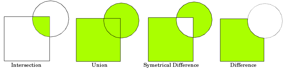
Spatial Joins and Overlays
Spatial Joins
A spatial join uses binary predicates
such as intersects and crosses to combine two GeoDataFrames based on the spatial relationship
between their geometries.
A common use case might be a spatial join between a point layer and a polygon layer where you want to retain the point geometries and grab the attributes of the intersecting polygons.
Types of spatial joins
Geopandas currently support the following methods of spatial joins. We refer to the left_df and right_df which are the correspond to the two dataframes passed in as args.
Left outer join
In a LEFT OUTER JOIN (how='left'), we keep all rows from the left and duplicate them if necessary to represent multiple hits between the two dataframes. We retain attributes of the right if they intersect and lose right rows that don't intersect. A left outer join implies that we are interested in retaining the geometries of the left.
Right outer join
In a RIGHT OUTER JOIN (how='right'), we keep all rows from the right and duplicate them if necessary to represent multiple hits between the two dataframes. We retain attributes of the left if they intersect and lose left rows that don't intersect. A right outer join implies that we are interested in retaining the geometries of the right.
Inner join
In an INNER JOIN (how='inner'), we keep rows from the right and left only where their binary predicate is True. We duplicate them if necessary to represent multiple hits between the two dataframes. We retain attributes of the right and left only if they intersect and lose all rows that do not. An inner join implies that we are interested in retaining the geometries of the left.
Example using Populated places
headers = {'User-Agent': 'Mozilla/5.0 (X11; Linux x86_64) AppleWebKit/537.36 (KHTML, like Gecko) Chrome/51.0.2704.103 Safari/537.36', 'Accept': 'text/html,application/xhtml+xml,application/xml;q=0.9,*/*;q=0.8'}

url = 'https://naturalearth.s3.amazonaws.com/10m_cultural/ne_10m_populated_places.zip'
r = requests.get(url, headers=headers)
populated_places = gp.read_file(io.BytesIO(r.content))
populated_places.head()
| SCALERANK | NATSCALE | LABELRANK | FEATURECLA | NAME | NAMEPAR | NAMEALT | NAMEASCII | ADM0CAP | CAPIN | ... | FCLASS_ID | FCLASS_PL | FCLASS_GR | FCLASS_IT | FCLASS_NL | FCLASS_SE | FCLASS_BD | FCLASS_UA | FCLASS_TLC | geometry | |
|---|---|---|---|---|---|---|---|---|---|---|---|---|---|---|---|---|---|---|---|---|---|
| 0 | 10 | 1 | 8.0 | Admin-1 capital | Colonia del Sacramento | None | None | Colonia del Sacramento | 0 | None | ... | None | None | None | None | None | None | None | None | None | POINT (-57.83612 -34.46979) |
| 1 | 10 | 1 | 8.0 | Admin-1 capital | Trinidad | None | None | Trinidad | 0 | None | ... | None | None | None | None | None | None | None | None | None | POINT (-56.90100 -33.54400) |
| 2 | 10 | 1 | 8.0 | Admin-1 capital | Fray Bentos | None | None | Fray Bentos | 0 | None | ... | None | None | None | None | None | None | None | None | None | POINT (-58.30400 -33.13900) |
| 3 | 10 | 1 | 8.0 | Admin-1 capital | Canelones | None | None | Canelones | 0 | None | ... | None | None | None | None | None | None | None | None | None | POINT (-56.28400 -34.53800) |
| 4 | 10 | 1 | 8.0 | Admin-1 capital | Florida | None | None | Florida | 0 | None | ... | None | None | None | None | None | None | None | None | None | POINT (-56.21500 -34.09900) |
5 rows × 138 columns
populated_places['ADM0_A3']
0       URY
1       URY
2       URY
3       URY
4       URY
       ...
7337    NZL
7338    NZL
7339    NZL
7340    IND
7341    IND
Name: ADM0_A3, Length: 7342, dtype: object
The number of places in each country is
number_pop_pl = populated_places.groupby(['ADM0_A3'])['geometry'].count()
number_pop_pl
ADM0_A3
ABW     1
AFG    33
AGO    49
ALB    26
ALD     1
       ..
WSM     1
YEM    20
ZAF    72
ZMB    34
ZWE    20
Name: geometry, Length: 225, dtype: int64
Imagine we did not have ADM0_A3
populated_places_noadm = populated_places.copy().drop(columns = ['ADM0_A3'])
populated_places_noadm.head()
| SCALERANK | NATSCALE | LABELRANK | FEATURECLA | NAME | NAMEPAR | NAMEALT | NAMEASCII | ADM0CAP | CAPIN | ... | FCLASS_ID | FCLASS_PL | FCLASS_GR | FCLASS_IT | FCLASS_NL | FCLASS_SE | FCLASS_BD | FCLASS_UA | FCLASS_TLC | geometry | |
|---|---|---|---|---|---|---|---|---|---|---|---|---|---|---|---|---|---|---|---|---|---|
| 0 | 10 | 1 | 8.0 | Admin-1 capital | Colonia del Sacramento | None | None | Colonia del Sacramento | 0 | None | ... | None | None | None | None | None | None | None | None | None | POINT (-57.83612 -34.46979) |
| 1 | 10 | 1 | 8.0 | Admin-1 capital | Trinidad | None | None | Trinidad | 0 | None | ... | None | None | None | None | None | None | None | None | None | POINT (-56.90100 -33.54400) |
| 2 | 10 | 1 | 8.0 | Admin-1 capital | Fray Bentos | None | None | Fray Bentos | 0 | None | ... | None | None | None | None | None | None | None | None | None | POINT (-58.30400 -33.13900) |
| 3 | 10 | 1 | 8.0 | Admin-1 capital | Canelones | None | None | Canelones | 0 | None | ... | None | None | None | None | None | None | None | None | None | POINT (-56.28400 -34.53800) |
| 4 | 10 | 1 | 8.0 | Admin-1 capital | Florida | None | None | Florida | 0 | None | ... | None | None | None | None | None | None | None | None | None | POINT (-56.21500 -34.09900) |
5 rows × 137 columns
How can we find the number of populated places in each country? Using spatial joins to identify which places are located in the country
Let's use gp.sjoin to get the the spatial join between both geodataframes
mysjoin = populated_places_noadm.sjoin(countries)
mysjoin
| SCALERANK | NATSCALE | LABELRANK_left | FEATURECLA | NAME_left | NAMEPAR | NAMEALT | NAMEASCII | ADM0CAP | CAPIN | ... | FCLASS_VN_right | FCLASS_TR_right | FCLASS_ID_right | FCLASS_PL_right | FCLASS_GR_right | FCLASS_IT_right | FCLASS_NL_right | FCLASS_SE_right | FCLASS_BD_right | FCLASS_UA_right | |
|---|---|---|---|---|---|---|---|---|---|---|---|---|---|---|---|---|---|---|---|---|---|
| 0 | 10 | 1 | 8.0 | Admin-1 capital | Colonia del Sacramento | None | None | Colonia del Sacramento | 0 | None | ... | None | None | None | None | None | None | None | None | None | None |
| 1 | 10 | 1 | 8.0 | Admin-1 capital | Trinidad | None | None | Trinidad | 0 | None | ... | None | None | None | None | None | None | None | None | None | None |
| 2 | 10 | 1 | 8.0 | Admin-1 capital | Fray Bentos | None | None | Fray Bentos | 0 | None | ... | None | None | None | None | None | None | None | None | None | None |
| 3 | 10 | 1 | 8.0 | Admin-1 capital | Canelones | None | None | Canelones | 0 | None | ... | None | None | None | None | None | None | None | None | None | None |
| 4 | 10 | 1 | 8.0 | Admin-1 capital | Florida | None | None | Florida | 0 | None | ... | None | None | None | None | None | None | None | None | None | None |
| ... | ... | ... | ... | ... | ... | ... | ... | ... | ... | ... | ... | ... | ... | ... | ... | ... | ... | ... | ... | ... | ... |
| 7337 | 8 | 10 | 8.0 | Populated place | Cambridge | None | None | Cambridge | 0 | None | ... | None | None | None | None | None | None | None | None | None | None |
| 7338 | 8 | 10 | 8.0 | Populated place | Kerikeri | None | None | Kerikeri | 0 | None | ... | None | None | None | None | None | None | None | None | None | None |
| 7339 | 8 | 10 | 8.0 | Populated place | Turangi | None | None | Turangi | 0 | None | ... | None | None | None | None | None | None | None | None | None | None |
| 7340 | 4 | 50 | 2.0 | Admin-1 capital | Leh | None | None | Leh | 0 | None | ... | None | None | None | None | None | None | None | None | None | None |
| 7341 | 4 | 50 | 50.0 | Admin-1 capital | Amaravati | None | None | Amaravati | 0 | None | ... | None | None | None | None | None | None | None | None | None | None |
7324 rows × 306 columns
sjoin by default uses the how=inner option
and keeps the geometries in the left dataframe
that intersect the right dataframe
We're not limited to using the intersection binary predicate. Any of the Shapely geometry methods that return a Boolean can be used by specifying the predicate kwarg.
You can change this to other options:
predicate='touches', or predicate='within', etc.
Let's compare results
mysjoin_pl = mysjoin.groupby(['ADM0_A3'])['geometry'].count()
mysjoin_pl
ADM0_A3
ABW     1
AFG    33
AGO    48
ALB    26
ALD     1
       ..
WSM     1
YEM    20
ZAF    72
ZMB    34
ZWE    20
Name: geometry, Length: 225, dtype: int64
number_pop_pl
ADM0_A3
ABW     1
AFG    33
AGO    49
ALB    26
ALD     1
       ..
WSM     1
YEM    20
ZAF    72
ZMB    34
ZWE    20
Name: geometry, Length: 225, dtype: int64
mysjoin_pl-number_pop_pl
ADM0_A3
ABW    0.0
AFG    0.0
AGO   -1.0
ALB    0.0
ALD    0.0
      ...
WSM    0.0
YEM    0.0
ZAF    0.0
ZMB    0.0
ZWE    0.0
Name: geometry, Length: 228, dtype: float64
compare_pl = pd.merge(mysjoin_pl, number_pop_pl, left_index=True, right_index=True, suffixes=['_sjoin', '_true'])
compare_pl
| geometry_sjoin | geometry_true | |
|---|---|---|
| ADM0_A3 | ||
| ABW | 1 | 1 |
| AFG | 33 | 33 |
| AGO | 48 | 49 |
| ALB | 26 | 26 |
| ALD | 1 | 1 |
| ... | ... | ... |
| WSM | 1 | 1 |
| YEM | 20 | 20 |
| ZAF | 72 | 72 |
| ZMB | 34 | 34 |
| ZWE | 20 | 20 |
222 rows × 2 columns
Where are there differences?
compare_pl.loc[compare_pl['geometry_sjoin']!=compare_pl['geometry_true']]
| geometry_sjoin | geometry_true | |
|---|---|---|
| ADM0_A3 | ||
| AGO | 48 | 49 |
| ARE | 7 | 8 |
| ARG | 156 | 158 |
| CAN | 254 | 255 |
| COL | 71 | 72 |
| CYP | 3 | 4 |
| DOM | 30 | 31 |
| GRL | 16 | 22 |
| KAZ | 95 | 96 |
| NAM | 28 | 27 |
| NOR | 35 | 34 |
| NZL | 53 | 52 |
| PAN | 13 | 14 |
| PER | 87 | 89 |
| PNG | 22 | 23 |
| PRT | 23 | 24 |
| USA | 768 | 769 |
Overlays
Spatial overlays allow you to compare two GeoDataFrames containing polygon or multipolygon geometries and create a new GeoDataFrame with the new geometries representing the spatial combination and merged properties. This allows you to answer questions like
How many people live within 100kms of a border and within 200kms of a populated place?
The basic idea is demonstrated by the graphic below but keep in mind that overlays operate at the dataframe level, not on individual geometries, and the properties from both are retained
Let us show how to answer the question above for one country, say Colombia
First, we need to get Colombia and its buffer
col = countries.loc[countries['ADM0_A3']=='COL'].reset_index(drop=True)
col = col.to_crs(cea)
We convert to CEA because we want to construct buffers around the border
col_buffer = col.copy()
col_buffer.geometry = col_buffer.boundary.buffer(100 * 1e3)
col_buffer.plot()
<Axes: >

Now, let's select populated places in Colombia
col_places = populated_places.loc[populated_places['ADM0_A3']=='COL'].reset_index()
col_places = col_places.to_crs(cea)
col_places.plot()
<Axes: >

col_places_buffer = col_places.copy()
col_places_buffer.geometry = col_places_buffer.buffer(200 * 1e3)
col_places_buffer.plot()
<Axes: >

To find the number of people within 100kms of a border and 200kms of a populated place we need to find the intersection of these two buffers
col_join = col_buffer.overlay(col_places_buffer)
col_join.head()
| featurecla | scalerank | LABELRANK_1 | SOVEREIGNT | SOV_A3_1 | ADM0_DIF | LEVEL | TYPE | TLC | ADMIN | ... | FCLASS_ID_2 | FCLASS_PL_2 | FCLASS_GR_2 | FCLASS_IT_2 | FCLASS_NL_2 | FCLASS_SE_2 | FCLASS_BD_2 | FCLASS_UA_2 | FCLASS_TLC_2 | geometry | |
|---|---|---|---|---|---|---|---|---|---|---|---|---|---|---|---|---|---|---|---|---|---|
| 0 | Admin-0 country | 0 | 2 | Colombia | COL | 0 | 2 | Sovereign country | 1 | Colombia | ... | None | None | None | None | None | None | None | None | None | POLYGON ((-7881837.774 673851.953, -7893451.99... |
| 1 | Admin-0 country | 0 | 2 | Colombia | COL | 0 | 2 | Sovereign country | 1 | Colombia | ... | None | None | None | None | None | None | None | None | None | POLYGON ((-9195952.170 1390669.459, -9195635.0... |
| 2 | Admin-0 country | 0 | 2 | Colombia | COL | 0 | 2 | Sovereign country | 1 | Colombia | ... | None | None | None | None | None | None | None | None | None | MULTIPOLYGON (((-8467942.672 809172.032, -8468... |
| 3 | Admin-0 country | 0 | 2 | Colombia | COL | 0 | 2 | Sovereign country | 1 | Colombia | ... | None | None | None | None | None | None | None | None | None | POLYGON ((-7932201.846 668361.394, -7941592.04... |
| 4 | Admin-0 country | 0 | 2 | Colombia | COL | 0 | 2 | Sovereign country | 1 | Colombia | ... | None | None | None | None | None | None | None | None | None | POLYGON ((-8053621.414 681606.911, -8061656.19... |
5 rows × 307 columns
col_join.plot()
<Axes: >
